Every Explanation Is a Simplification
SHAP plots, saliency maps, and attention visualisations look like evidence. But evidence of what?

This is Part 1 of a two-part series on explainability and assurance. Part 2 covers the mathematical limits of explainability and what they mean for regulation.
Explainability of AI systems has quickly become a compliance obligation for organisations developing, procuring, and deploying AI systems. The EU AI Act requires that high-risk AI systems be designed so that their operation is “sufficiently transparent” for deployers to interpret and use outputs appropriately.[1] NIST’s AI Risk Management Framework lists explainability as a core characteristic of trustworthy AI.[2] And the UK’s AI assurance roadmap expects organisations to demonstrate that their systems can be understood by relevant stakeholders.[3]
Understandably, when organisations are shown the stick rather than the carrot, they respond by generating explanations. SHAP plots appear in model cards. Saliency maps accompany clinical decision support outputs. Attention visualisations show up in technical documentation. These artefacts look like evidence of compliance. But what are they, structurally? What do they actually tell you about the model, and what do they leave out?
This matters because an explanation that looks informative but misleads is worse than no explanation at all. It can create the appearance of understanding where none exists. And if that explanation ends up in an assurance case as evidence for a transparency or explainability claim, the argument it supports is built on weaker foundations than anyone involved realises.
Explanation as compression
Here is a useful way to think about what any explanation method is doing:
An explanation compresses a model’s behaviour into something simpler.
A modern machine learning model might have millions of parameters encoding a complex, nonlinear function from inputs to outputs. No human can look at those parameters and understand what the model does. So explanation methods produce a smaller, more interpretable object (or model) that approximates some aspect of the model’s behaviour.
This framing comes from information theory. Rao (2025) formalises it using a measure known as Kolmogorov complexity.[4] But you do not need the formalism to grasp the core point. An explanation is a compression, and compression, by definition, discards information. With this in mind, we then need to consider under what conditions the remaining information is reliable, and whether those conditions hold for a specific deployment context.
Different explanation methods compress differently, which means they trade away different things. Three broad families illustrate this.
Perturbation-based methods: explaining a different model
Methods like LIME and SHAP (in its model-agnostic form) work by probing the model from the outside.[5] They perturb the input (e.g. changing features, masking regions, adding noise) and observe how the model’s output changes. From these perturbation-output pairs, they fit a simpler model that locally approximates the original model’s behaviour.
The output you see (e.g. a bar chart of feature importances, highlighted regions of an image) describes this simpler model’s behaviour, not the original model’s internal reasoning. This is not a subtle technicality. The explanation describes a surrogate model (i.e. an interpretable approximation fitted to sampled perturbations). If the surrogate and the model disagree in ways that the sampling did not catch, the explanation will be wrong and there is no built-in mechanism to detect this. Some SHAP variants partially address this gap, but formal error guarantees for general models remain provably difficult to obtain.[6]
Consider a clinical decision support system that flags patients as high-risk for a particular condition based on pathology results. A LIME explanation might report that two biomarkers were the most important features for a specific patient’s risk score. But if the actual model relies on a nonlinear interaction between those biomarkers and a third variable (e.g. the patient’s age), and the perturbation sampling did not explore that interaction region densely enough, the linear surrogate will miss it entirely. The explanation will look clean and confident. It will also be incomplete in a way that matters clinically.
The figure below illustrates this with a simplified example. Imagine a screening model that classifies patients as low risk or high risk based on two biomarker measurements. The model has learned a curved decision boundary (the dashed blue line) separating the two classes. A specific patient of interest sits above the boundary, classified as high risk.
To explain this classification, LIME generates perturbation samples in the local neighbourhood around that patient (the dashed circle), feeds them to the model, and fits a straight line (the coral surrogate) that approximates the model’s boundary locally. Where the straight surrogate and the curved boundary diverge is what we can call the “fidelity gap”: the region where the surrogate would give a different answer than the actual model. Any patient falling in this gap would be mischaracterised by the explanation.
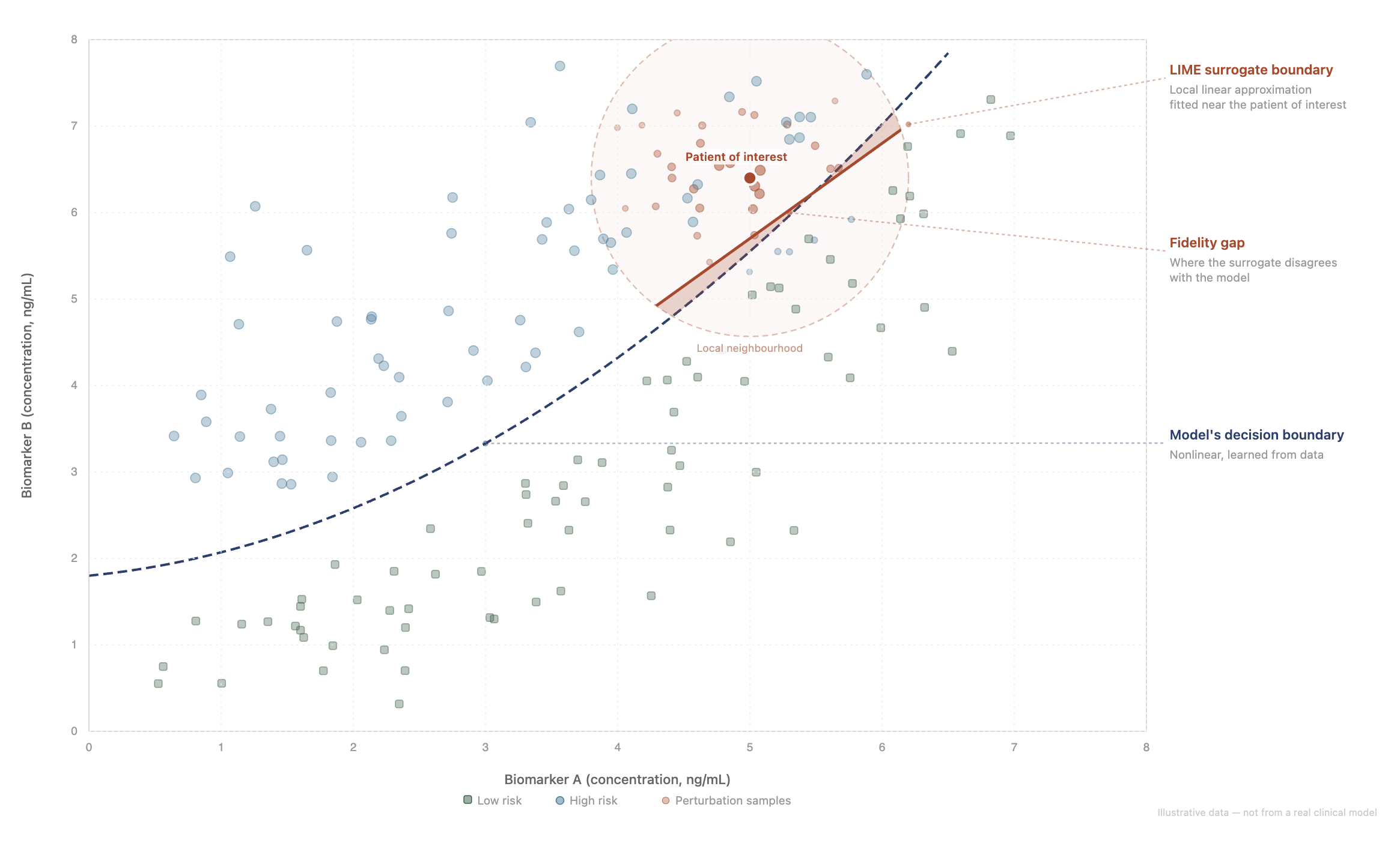
Figure 1. A LIME explanation fits a local linear surrogate near a specific input. The gap between the surrogate and the model’s actual decision boundary is the fidelity risk. Illustrative data — not from a real clinical model.
Notice that the surrogate exists only within the local neighbourhood. LIME does not claim global accuracy. But within that neighbourhood, the gap between the straight line and the curve is real, rarely quantified in practice, and invisible in a standard LIME output. The bar chart of feature importances you see in practice does not tell you how large this gap may be.
Gradient-based methods: exact at a point, fragile everywhere else
Gradient-based methods (e.g. Grad-CAM, Integrated Gradients, Layer-wise Relevance Propagation) take a different approach.[7] Instead of probing the model from the outside, they use the model’s internal mathematics. Specifically, they compute the gradient of the model’s output with respect to its inputs (i.e. a measure of how much each input feature would change the output if nudged slightly).
This has an important advantage over perturbation-based methods, because the gradient is a property of the actual model, not a fitted surrogate. There is no fidelity gap in the same sense as perturbation methods. The gradient tells you exactly how the model behaves at one specific point.
But as you may expect, that precision comes with trade-offs:
First, scope: the gradient describes infinitesimally local behaviour. It tells you the slope of the model’s decision surface at one point but says nothing about the model’s behaviour even slightly away from that point. For a highly nonlinear model, the gradient at a specific input may be a poor guide to why the model made its decision. The relevant structure might be in the curvature or the interactions between features, neither of which the gradient captures.
Second, stability: research has shown that many gradient-based methods fail a basic sanity check called input invariance.[8] A constant shift applied to all inputs, such as a transformation that does not change the model’s predictions, can dramatically change the explanations these methods produce. Worse, researchers have demonstrated that adversarial perturbations can be deliberately injected to produce misleading explanations while leaving the model’s outputs unchanged. If a trivial input transformation changes the explanation without changing the prediction, the explanation does not reliably reflect what the model computes.
For assurance, the trade-off is scope and stability. The gradient is exact at a point but potentially unrepresentative, and it may not be stable under realistic input variation. If you cannot demonstrate that stability with evidence, the explanation is not strong enough to support a claim in an assurance case.
Attention-based methods: real internals, ambiguous meaning
In transformer architectures, which are the basis for most large language models and an increasing share of vision systems, attention mechanisms determine how the model weighs different parts of the input when producing an output. Attention maps are sometimes presented as explanations, such as “the model was paying attention to these words” or “the model focused on this region of the image.”
Unlike gradient and perturbation methods, attention weights are genuine model internals. They are computed during the model’s forward pass (the computation the model runs each time it processes an input and produces a prediction), not derived after the fact. This makes them computationally cheap and seemingly authoritative.
But the interpretation is more fraught than it appears. Research on attention faithfulness has found that raw attention weights show the magnitude of a feature’s influence but not its direction.[9] A feature with high attention may be strongly supporting the model’s prediction or strongly suppressing it. The attention weight alone cannot tell you which.
Liu et al. (2022) found faithfulness violation rates of 28–48% for raw attention across multiple architectures and datasets, meaning that for roughly a third to nearly half of the most-attended features, the direction of influence was the opposite of what a naive reading of the attention map would suggest. The violation rates were worst for transformer architectures. Gradient-weighted attention variants substantially reduce this problem, but raw attention maps, which are what most practitioners see and share, do not.
Compression has consequences
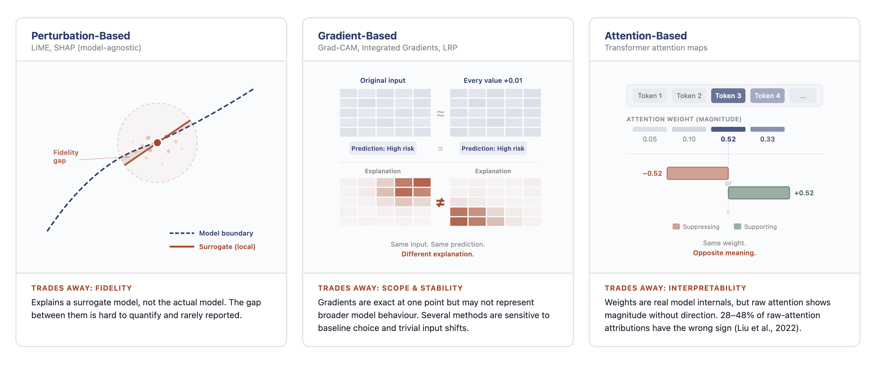
Figure 2. Three explanation families, three trade-offs. Every method simplifies differently, and every simplification discards something.
These three families do not exhaust the field. Instance-based methods (e.g. prototype networks and nearest-neighbour approaches), representation analysis techniques (e.g. dimensionality reduction applied to internal representations), and causal analysis methods each work differently and have their own trade-offs.[10] But the structural point holds across all of them:
Every explanation method produces a simplified view of model behaviour, and every simplification discards something.
To put it another way, simplification is inherent to explanation. You cannot explain a complex system without compressing it, and compression always loses information. But organisations generating explanations for compliance or assurance purposes still need to ask important questions about what their assurance case requires:
What specifically does this explanation method trade away? (Fidelity? Scope? Interpretability of the output?)
Under what conditions is the simplification reliable?
What would cause those conditions to break? (Distribution shift? Adversarial inputs? Model updates?)
What evidence do you have that those conditions currently hold?
Without answers to these questions, the SHAP plot in your model card and the saliency map in your technical report may look like evidence of compliance, but their evidential value remains unexamined.
I want to be clear that this is not an argument against using explanation methods. Rather, it’s an argument for treating them with the same discipline you would apply to any other piece of evidence in a structured assurance case. An explanation method has assumptions, limitations, and conditions of validity. Documenting these is what turns an output into evidence.
What comes next
If every explanation is a simplification, a natural follow-up is:
How much simplification can you get away with? Is there a point where an explanation is too simple to be faithful, regardless of how much computational effort you invest?
Next week I will look at these questions in further detail, and I will walk through what the mathematics of compression tells us about the hard limits of explainability, why no regulation can simultaneously demand powerful AI and simple, accurate explanations, and what those limits mean for anyone writing an assurance case that includes an explainability claim.
This is the third edition of Burden of Proof, and Part 1 of a two-part series on explainability and assurance. Each week, I take one development in AI assurance and work through what it means in practice. If you found this useful, subscribe to get future posts delivered to your inbox.
EU AI Act, Article 13 — Transparency and provision of information to deployers. High-risk AI systems must be designed so that their operation is “sufficiently transparent to enable deployers to interpret the system’s output and use it appropriately.”↩︎
NIST, AI Risk Management Framework, January 2023. Explainability and interpretability are identified as characteristics of trustworthy AI under the “Explainable and Interpretable” category.↩︎
DSIT, Trusted Third-Party AI Assurance Roadmap, September 2025.↩︎
Rao (2025), The Limits of AI Explainability: An Algorithmic Information Theory Approach. Rao formalises explanations as compressed representations and establishes both a Complexity Gap Theorem and a Regulatory Impossibility Theorem. The regulatory implications are the subject of Part 2 of this series.↩︎
Ribeiro, Singh, and Guestrin (2016), “Why Should I Trust You?”: Explaining the Predictions of Any Classifier, introduced LIME. Lundberg and Lee (2017), A Unified Approach to Interpreting Model Predictions, introduced SHAP.↩︎
TreeSHAP (Lundberg et al., 2020) computes exact Shapley values for tree-based models without a surrogate, but faces different issues with correlated features. BayesSHAP (Slack et al., 2021, Reliable Post hoc Explanations: Modeling Uncertainty in Explainability, NeurIPS) provides Bayesian credible intervals on SHAP coefficients, partially addressing the uncertainty gap. Van den Broeck et al. (2022) establish that computing exact SHAP values is #P-hard in general, meaning formal error guarantees for approximations are provably difficult to obtain.↩︎
Selvaraju et al. (2017), Grad-CAM: Visual Explanations from Deep Networks via Gradient-based Localization. Sundararajan, Taly, and Yan (2017), Axiomatic Attribution for Deep Networks (Integrated Gradients). Bach et al. (2015), On Pixel-Wise Explanations for Non-Linear Classifier Decisions by Layer-Wise Relevance Propagation (LRP).↩︎
Kindermans et al. (2017), The (Un)reliability of Saliency Methods. A constant shift to inputs (which does not change the model’s output) produces dramatically different saliency maps for Gradient × Input, Integrated Gradients, and LRP. Note that Grad-CAM was not tested in this study; it operates on intermediate convolutional feature maps rather than input-level gradients and has a different vulnerability profile. For Integrated Gradients specifically, the fragility is tied to baseline (reference point) selection rather than an intrinsic instability of the gradient computation.↩︎
Liu et al. (2022), Rethinking Attention-Model Explainability through Faithfulness Violation Test, Proceedings of the 39th International Conference on Machine Learning (ICML). The authors measure polarity consistency — whether the direction of a feature’s influence matches what the explanation suggests. Raw attention explanations showed violation rates of 28–48% depending on architecture and dataset, with transformer-based models performing worst. Gradient-weighted attention variants (e.g. AttGrad) reduce violation rates to single digits, suggesting that the polarity problem is addressable but is not addressed by raw attention weights alone.↩︎
For a taxonomy of explanation method types and their explanation targets, see the TEA Techniques dataset, which categorises 55 explainability techniques across nine method types and six explanation target categories.↩︎